Duncan Watts’ “Small Worlds” α-model

How to run a CDF Player simulation
download Watts_alpha_Model.cdf
download Watts_alpha_Model.nb (Mathematica notebook)

Overview

This is a Mathematica simulation of Watts’ “Small Worlds” $\alpha$ -model.
The meaning of the parameters used in the model is:

$n$ : total number of nodes of the graph
$k_f$ : final average degree of the graph (average number of connections for each node)
$\alpha$ : tunable parameter to regulate between the caveman ( $\alpha \to 0$ ) vs. solaria ( $\alpha \to \infty$ ) propensities for new connections.
$p$ : a baseline (small) probability for the creation of a random connection between any couple of nodes

This model can be useful to understand how a social network can build up and develop, starting from the simplest connected network (ring) and using some simple assumptions, such as “the friends of my friends are likely to become my friends too“.
For different values of the $\alpha$ parameter the network evolution will change its connection propensity: from one in which only mutual friends drive new connections to one in which new connections are mainly created by chance.
The mean clustering coefficient and the mean graph distance (showed above the graph image) are measures of the clusters formation (highly interconnected subgraphs) and of the average length of connections between any two nodes (along the shortest path) for all the pairs of network nodes.
According to Watts a small world network is characterized by both high clustering and short average distance and this situation may occurs for a certain range of values of the $\alpha$ parameter.
This phenomenon is also the basis of the much more popular theory of the six degree of separation. According to this theory there is a relatively very short average distance (just 6 steps) in the huge network of the whole population of our world, that sums up to more than 7 billions nodes (people) in 2014. Yet, despite the relatively small distance, the present social structure of the set of world citizens is not that of a random graph (that would easily explain the short distance between any two nodes) but rather that of highly clustered network with geographical, linguistic, economic or cultural interconnected communities.

Usage of the simulation

Changing the overall graph parameters ( $n$ , $k_f$ , $\alpha$ , $p$ ) triggers the whole graph to be recalculated, so it may take some time for the higher values of $n$ and or $k_f$ .
The $t$ parameter, instead, just shows the steps through which the graph is built until it’s final degree (total number of nodes connections) and doesn’t require a recalculation of the whole graph (so it’s rather quick).

The model

The rationale of the $\alpha$ -model and the role of its relevant parameters ( $n$ , $k_f$ , $\alpha$ , $p$ ) are explained in the book;

Duncan J. Watts – Small Worlds: The Dynamics of Networks between Order and Randomness
[Princeton University Press – 1999]

There’s a free preview snippet by the editor at Google Books that explains it (from page 44 to page 48).
It’s here (click on page 46).

The parameters used in the model are:

$\boxed{n}$ : total number of nodes in the network.

$\boxed{k_f}$ : the average number of connections for each node (or average number of friends for each member of the community) to be reached at the end of the network construction. The parameters $n$ and $k_f$ regulate the final total number of edges in the graph: $M = \frac{{k_f \cdot n}}{2}$ .
A fully connected graph (in which each node has a direct connection with each other node) will have the maximum ${k_f}$ for a given $n$ , with ${k_f} = n - 1$ and $M = \left( {\begin{array}{*{20}{c}}n \\2\end{array}} \right) = \frac{{n \cdot \left( {n - 1} \right)}}{2}$

$\boxed{\alpha}$ ( $0 \le\alpha\le \infty$ ) is a tunable parameter to regulate between the caveman ( $\alpha \to 0$ ) vs. solaria ( $\alpha \to \infty$ ) propensities for new connections.
The caveman community will tend to establish new links only between inhabitants of the same cave so that members of cave A will soon be interconnected and form a cluster of friends. At the same time there will be a very small probability that a caveman of cave A will connect with another caveman of cave B. So the caveman community could be described by the sentence “Everybody you know knows everybody else you know and no one else (or almost no every one else) ”
On the other end there’s the solaria community. Its members could be thought of like modern chat-rooms users that can connect randomly with every other world citizen (and not mainly with just friends of friends). In this community the influence of current friendships over new friendships is very small and new friendships (links) are mainly governed by chance.

$\boxed{p}$ ( $0 \le p \le 1$ ) is the baseline probability for the creation of a random connection between any couple of nodes. In this model $p$ must be considered a very small probability (say 0.001 or even less for bigger networks) that gets relevance only when the $\alpha$ parameter has such values to make the number of friends of friends irrelevant for creating a new connection.

Duncan Watts’ $\alpha$ -model is based on the following loop algorithm:
1. At step (time) $t$ examine the graph at the previous step $t-1$ and, for each couple of nodes $i$ and $j$ (that are not already directly connected) calculate:
• $m_{ij}$ : number of nodes which are adjacent both to $i$ and $j$ (mutual friends of i and j)
• $k$ : average degree of the network at time $t-1$ , that is the average number of connections (friends) for every node at time $t-1$ .
2. Calculate the propensity matrix ${R_{ij}}$ according to the following formula:
$\boxed{{R_{ij}}= \left\{ {\begin{array}{*{20}{l}}1&{ & & {m_{ij}} \ge {k}}\\{{{\left( {\frac{{{m_{ij}}}}{{{k}}}} \right)}^\alpha }\cdot\left( {1 - p} \right) + p}&{ & & 0 < {m_{ij}} < {k}}\\p&{ & & {m_{ij}} = 0}\end{array}} \right.}$
The propensity matrix ${R_{ij}}$ will then be rescaled and normalized to a probability matrix ${P_{ij}}$ , with ${P_{ij}} = {{{R_{ij}}} \mathord{\left/ {\vphantom {{{R_{ij}}} {\sum\limits_{j = 1}^n {{R_{ij}}} }}} \right. \kern-\nulldelimiterspace} {\sum\limits_{j = 1}^n {{R_{ij}}} }}$ so that $\sum\limits_{j = 1}^n {{P_{ij}} = 1}$ .
In this matrix ${P_{ij}}$ can be interpreted as the probability that node i will connect with node j.

Above ${R_{ij}}$ rule translates in the following two extremes.
For pure caveman communities ( $\alpha=0$ ) it will be:
$\mathop {{R_{ij}}}\limits_{\alpha \to 0} = \left\{ {\begin{array}{*{20}{l}}1&{ & & {m_{ij}} > 0}\\p&{ & & {m_{ij}} = 0}\end{array}} \right.$
which means that any couple of people with just one single mutual friend will have a much greater probability to become connected than people without any mutual friends (since $p$ is a small number)
On the other extreme, for pure solaria communities ( $\alpha \to \infty$ ), it will be:
$\mathop {{R_{ij}}}\limits_{\alpha \to \infty } = \left\{ {\begin{array}{*{20}{l}}1&{ & & {m_{ij}} \ge {k_{t - 1}}}\\p&{ & & {m_{ij}} < {k_{t - 1}}}\end{array}} \right.$
which means that, unless the nodes i and j have reached a critical threshold of mutual friends, the probability of their connection will be the same as the probability of connection between two nodes with no mutual friends at all.
The critical threshold for the number of mutual friends that can actually trigger the connection is set at the rather high value of the current average degree of the network. This can be interpreted considering that, even in a solaria community, if two unlinked people have all their current friends in common (and that’s rather unlikely to happen since there will normally be, for the nodes i and j several friends that are not in common) than they can’t really avoid knowing each other.

For intermediate (and more realistic) forms between the pure caveman and the pure solaria communities, the following picture shows the relations between the “propensity to become friends” and the “mutual friends as a fraction of total friends” for different possible values of the $\alpha$ parameter.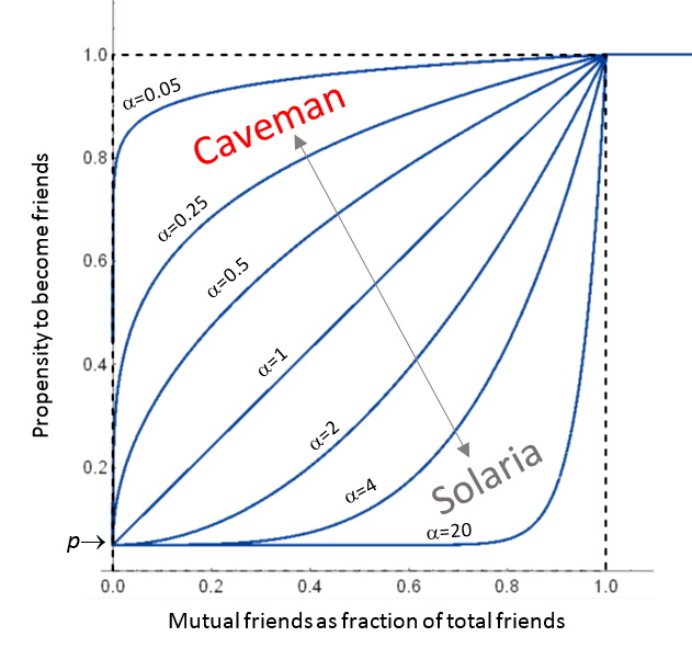

The $\alpha$ -model is a variant of the more known (and much more simple) $\beta$ -model (also known as Watts–Strogatz model). Anyway the $\alpha$ -model seems much more interesting for its intrinsic dynamic characteristics that can help to understand and visualize the network evolution.

The algorithm

The process for building the final graph is based on a loop.
In each cycle of the loop a new edge will be added until the final number of edges $M$ is reached ( $M = \frac{{k_f \cdot n}}{2}$ ).
The initial condition for the network is a topological ring, in which each node connects to exactly two other nodes, forming a single continuous pathway between linked nodes.

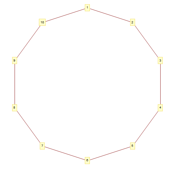Note: even if this particular choice of the initial condition could seem arbitrary and have some unwanted effect in the subsequent evolution of the network, it has however the following motivations and advantages:
• The initial graph is connected (each node is reachable from each other node) and will stay connected in the following steps (since the algorithm will just add new edges and not delete existing ones). This will make it possible to calculate the average distance between any two nodes, avoiding the possible case in which disconnected subgraphs (islands) builds up. That circumstance could be possible in some social network (and surely that was a typical situation of the social world networks of the past) but that wouldn’t properly reflect the interconnectedness of our present world.
• It has a minimal structure: no vertex is special or different from any other vertex in terms of number of connections.
• It’s minimally connected: it has the minimum number of edges for a connected graph with the minimal structure requirement.
Duncan J. Watts calls this initial condition a substrate and explains how this ring choice for the substrate is supposed to have the minimal possible impact on the evolution of the global network (assuming that the final global network must have a global interdependence characteristic).

Since the initial condition is a graph with $n$ nodes and $n$ edges, in order to reach the final number of edges ( $M = \frac{{k_f \cdot n}}{2}$ ) there will be $M-n$ iterations in the loop.

The generic $t^{th}$ iteration of the loop will go through the following steps:

• Choose a vertex i.
• For every other vertex j, compute ${R_{ij}}$ and ${P_{ij}}$ .
These two matrices will depend on the values of the general (fixed) parameters $\alpha$ and $n$ but also on the dynamic values of the matrix $m_{ij}$ and on the value of $k$ calculated form the adjacency matrix built at the previous step $t-1$ .
• The vertex i will then connect with another randomly chosen vertex j. Even if this choice is random it will be weighted by the $P_{ij}$ probabilities.
• When the link ij is established the symmetric adjacency matrix is updated (placing a 1 at positions ij and ji).

The vertices i are chosen in random order, but once a vertex has been allowed to choose e new neighbour (j), it may not choose again until all other vertices have taken their turn.
This democratic procedure limits the possibility, for each node, to be selected more frequently than the others for choosing a partner (since it must wait its turn) but doesn’t prevent some node to be chosen arbitrarily often by the other nodes. This means that there will be a nonzero variance in the degree $k_i$ of the graph’s nodes and that some node can assume the role of a local hub (with its degree $k_i$ higher than the graph mean degree k) in the network evolution.
On the other hand the less frequently chosen nodes will anyway (even if more slowly) increase their number of friends when their turn to choose comes, and they’ll go from 2 friends (initial condition) to a minimum final value of $1+\frac{k_f}{2}$ (in the case they are never chosen by the other nodes).

Final considerations

Watts’ conjecture is that:

There exist a class of graphs that are highly clustered yet have characteristic length and length scaling properties equivalent to random graphs. These are called small-world graphs. [p.58]

To verify it Watts used his $\alpha$ -model to run simulations that seem to confirm (with high probability) above conjecture.
The demonstration presented in this page (replicating the $\alpha$ -model in a small scale) is rather limited in the number of nodes it can manage (in a reasonable time), and so it’s not really suitable to give unquestionable answers to Watts’ conjecture.
Nonetheless it can be useful to better understand the $\alpha$ -model and the possible insurgence of small-world networks in the real world.

References

♦ from http://en.wikipedia.org:
Graph theory, Six degrees of separation, Small-world network

♦ from http://www.youtube.com:
The Science of Six Degrees of Separation
A video by (the great) Veritasium explaining the basic principles of the “Six degrees” theory.

♦ from other sites:
Reka Albert, Albert-Laszlo Barabasi: Statistical mechanics of complex networks (pdf – arxiv.org)

Duncan J. Watts, Steven H. Strogatz: Collective dynamics of ‘small-world’ networks (pdf – Nature 393, 440-442 – 4 June 1998)

The story of networks (blog – http://www.digitaltonto.com)

David Easley, Jon Kleinberg: Networks, Crowds, and Markets: Reasoning About a Highly Connected World – Cambridge University Press – 2010. There is a complete pre-publication draft (pdf) downloadable at above authors’ page.

from you tube

♦ books:
Duncan J. Watts – Small Worlds: The Dynamics of Networks between Order and Randomness – Princeton University Press – 1999

Steven Strogatz – Sync – Penguin Books – 2003

Author: Luca Moroni – October 2014

worlds of math & physics

Duncan Watts’ “Small Worlds” alpha model